Here describes Optical System Conventions and Definitions and defines terminology, which are common in the optics industry, however there may be some important differences.
Angular Magnification
The ratio of the paraxial image space chief ray angle to the paraxial object space chief ray angle. The angles are measured with respect to the paraxial entrance and exit pupil locations.
Apodization refers to the uniformity of illumination in the entrance pupil of the system. By default, the pupil is always illuminated uniformly. However, there are times when the pupil should have a non-uniform illumination. For this purpose, the design software supports pupil apodization, which is a variation of amplitude over the pupil.
Three types of pupil apodization are supported: uniform, Gaussian, and tangential. For each type (except uniform), an apodization factor determines the rate of variation of amplitude in the pupil.
Back Focal Length
Some software defines the back focal length as the distance along the Z axis from the last surface made of glass to the paraxial image surface for the object at infinite conjugates.
Note that if the image space is not in air (the Material column of the Image surface
contains a Material name), the reported back focal length will be the distance from the
Image surface to the paraxial image location for the object at infinite conjugates.
If no surfaces are made of glass, the back focal length is the distance from surface 1 to the paraxial image surface for the object at infinite conjugates.
Cardinal Planes
The term cardinal planes refers to those special conjugate positions where the object and image surfaces have a specific magnification. The point where the plane intersects the optical axis is the cardinal point corresponding to that cardinal plane. The cardinal planes include the principal planes, where the lateral magnification is +1, the anti-principal planes, where the lateral magnification is -1, the nodal planes, where the angular magnification is +1, the anti-nodal planes, where the angular magnification is -1, and the focal planes, where the magnification is 0 for the image space focal plane and infinite for the object space focal plane.
Except for the focal planes, the cardinal planes are conjugates with each other, that is, the image space principal plane is conjugate with the object space principal plane, etc. If the lens has the same index in both object space and image space, the nodal planes are identical to the principal planes.
Chief Ray
If there is no vignetting, and there are no aberrations, the chief ray is defined to be the ray that travels from a specific field point, through the center of the entrance pupil, and on to the image surface. Note that without vignetting or aberrations, any ray passing through the center of the entrance pupil will also pass through the center of the stop and the exit pupil.
When vignetting factors are used, the chief ray is then considered to be the ray that passes through the center of the vignetted pupil, which means the chief ray may not necessarily pass through the center of the stop.
If there are pupil aberrations, and there virtually always are, then the chief ray may pass
through the center of the paraxial entrance pupil (if ray aiming is off) or the center of the stop (if ray aiming is on), but generally, not both.
If there are vignetting factors which decenter the pupil, then the chief ray will pass through the center of the vignetted entrance pupil (if ray aiming is off) or the vignetted stop surface (if ray aiming is on).
The common convention used is that the chief ray passes through the center of the vignetted pupil, while the principal ray passes through the center of the unvignetted stop. Most the design software never uses the principal ray. Most calculations are referenced to the chief ray or the centroid. Note the centroid reference is generally superior because it is based upon the aggregate effect of all the rays that actually illuminate the image surface, and not on the arbitrary selection of
one ray which is “special”.
Coordinate Axes
The optical axis is the Z axis, with the initial direction of propagation from the object being the positive Z direction. Mirrors can subsequently reverse the direction of propagation. The coordinate system is right handed, with the sagittal X axis being oriented “into” the monitor on a standard layout diagram. The tangential Y axis is vertical. The direction of propagation is initially left-to-right, down the positive Z axis. After an odd number of mirrors the beam physically propagates in a negative Z direction. Therefore, all thicknesses after an odd number of mirrors should be negative in most of Optical System Conventions and Definitions.
Diffraction Limited
The term diffraction limited implies that the performance of an optical system is limited by the physical effects of diffraction rather than imperfections in either the design or fabrication. A common means of determining if a system is diffraction limited is to compute or measure the optical path difference. If the peak to valley OPD is less than one quarter wave, then the system is said to be diffraction limited.
There are many other ways of determining if a system is diffraction limited, such as Strehl ratio, RMS OPD, standard deviation, maximum slope error, and others. It is possible for a system to be considered diffraction limited by one method and not diffraction limited by another method.
On some plots, such as the MTF or Diffraction Encircled Energy, the diffraction
limited response is optionally shown. This data is usually computed by tracing rays from a reference point in the field of view. Pupil apodization, vignetting, F/#’s, surface apertures, and transmission may be accounted for, but the optical path difference is set to zero regardless of the actual (aberrated) optical path.
For systems which include a field point at 0.0 in both x and y field specifications (such as 0.0 x angle and 0.0 y angle), the reference field position is this axial field point. If no (0, 0) field point is defined, then the field coordinates of field position 1 are used as the reference coordinates instead.
Edge Thickness
Some design software defines the edge thickness of a surface as:

Where Zi is the sag of the surface, Zi+1 is the sag of the next surface, and Ti is the axial
thickness of the surface. The sag values are computed at the +y clear semi-diameter or semidiameter of their respective surfaces; Note that edge thickness is computed for the +y radial aperture, which may be inadequate if the surface is not rotationally symmetric, or if surface apertures have been placed upon either of the surfaces.
Edge thickness solves use a slightly different definition of edge thickness. For edge thickness solves only, the sag of the i+1 surface is computed at the clear semi-diameter or semidiameter of surface i. This method avoids a possible infinite loop in the calculation, since changing the thickness of surface i may alter the clear semi-diameter or semi-diameter of surface i+1, if the latter clear semi-diameter or semi-diameter is in “automatic” mode and the value is based upon ray tracing.
Effective Focal Length
The Effective Focal Length (or Equivalent Focal Length) is the distance from the secondary principal plane to the paraxial focal plane. The secondary principal plane is calculated by tracing an on-axis parabasal ray from infinity and determined using the parabasal’s image space marginal ray angle.
The Effective Focal Length is calculated in many softwares based on equation below:

Where K is the power of system, F is the Effective Focal Length, n’ are the index of materials in image space, f’ are the secondary focal lengths in image space.
Note the secondary focal length (f’) is list as “Effective Focal Length (in Image Space)” in the Prescription Data, which is Effective Focal length multiplied by the refractive index in image space. For example, below figure displayed sample system EFLs in air and water image space:

Entrance Pupil Diameter
The diameter in lens units of the paraxial image of the stop in object space.
Entrance Pupil Position
The paraxial position of the entrance pupil with respect to the first surface in the system. The first surface is always surface 1, not the object surface, which is surface 0.
Exit Pupil Diameter
The diameter in lens units of the paraxial image of the stop in image space.
Exit Pupil Position
The paraxial position of the exit pupil with respect to the image surface.
Note the software will first try to trace real parabasal rays to calculate the exit pupil position in sequential mode. If, however, the central ray can’t be traced, we switch to paraxial rays to estimate the pupil position. The usage of parabasal rays may sometimes give unexpected result if there are some unusual components in the system. For example, this can happen if users make an User Defined surface which has some kind of discontinuous behavior of the surface as the rays intersect close to the vertex.
Field Angles and Heights
Field points may be specified as angles, object heights (for systems with finite conjugates), paraxial image heights, or real image heights. Field angles are always in degrees. The angles are measured with respect to the object space z axis and the paraxial entrance pupil position on the object space z axis. Positive field angles imply positive slope for the ray in that direction,and thus refer to negative coordinates on distant objects. The software converts x field angles
(αx) and y field angles (αy) to ray direction cosines using the following formulas:

where l, m, and n are the x, y, and z direction cosines.
If object or image heights are used to define the field points, the heights are measured in lens units.
When paraxial image heights are used as the field definition, the heights are the paraxial image coordinates of the primary wavelength chief ray on the paraxial image surface, and if the optical system has distortion, then the real chief rays will be at different locations.
When real image heights are used as the field definition, the heights are the real ray
coordinates of the primary wavelength chief ray on the image surface.
When angles are used as the field definition, the maximum radial field is used to calculate the normalization of all defined field points. For this reason, the maximum radial field is also called the normalization angle in many Optical System Conventions and Definitions.
Float by Stop Size
Float by stop size is one of the system aperture types supported by some design softwares. This phrase refers to the fact that the entrance pupil position, object space numerical aperture, image space F/#, and stop surface radius all are specified if just one of them is specified. Therefore, setting the stop radius, and then allowing the other values to be whatever they are, is a perfectly valid way of defining the system aperture. It is particularly handy when the stop surface is a real, unchangeable aperture buried in the system, such as when designing null corrector optics.
Ghost Reflections
Ghost reflections are spurious, unwanted images formed by the small amount of light which reflects off of, rather than refracts through a lens face. For example, the multiple images of the aperture stop visible in photographs taken with the sun in the field of view are caused by ghost reflections. Ghost images can be problematic in imaging systems and in high power laser systems.
Glasses
Glasses are entered by name in the glass column.
Blanks are treated as air, with unity index. Mirrors can be specified by entering “MIRROR” for the glass type, although this name will not appear in the glass catalog. The index of refraction of the mirror space is always equal to the index of refraction of the media before the mirror.
If a surface or object has the material type MIRROR, light will only be reflected. The transmitted part will be ignored. The behavior is different depending on whether a coating has been specified:
l If no coating is specified, the surface is assumed to be coated with a thick layer of
aluminum, with an index of refraction 0.7 – 7.0i. The aluminum layer is assumed to be
thick enough that no light propagates past the layer. This means that an uncoated mirror surface has a reflectivity of less than 1 although the exact value will depend on the polarization of the rays.
If a coating is specified, the reflectivity will be that of the coating.
Hexapolar Rings
Some software usually selects a ray pattern for you when performing common calculations such as spot diagrams. The ray pattern refers to how a set of rays is arranged on the entrance pupil.The hexapolar pattern is a rotationally symmetric means of distributing a set of rays. The hexapolar pattern is described by the number of rings of rays around the central ray. The first ring contains 6 rays, oriented every 60 degrees around the entrance pupil with the first ray starting at 0 degrees (on the x-axis of the pupil). The second ring has 12 rays (for a total of 19, including the center ray in ring “0”). The third ring has 18 rays. Each subsequent ring has 6 more rays than the previous ring.
Many features which require a sampling parameter to be specified (such as the spot diagram) use the number of hexapolar rings as a convenient means of specifying the number of rays. If the hexapolar sampling density is 5, it does not mean that 5 rays will be used. A sampling of 5 means 1 + 6 + 12 + 18 + 24 + 30 = 91 rays will be used.
Image Space F/#
Image space F/# is the ratio of the paraxial effective focal length calculated at infinite
conjugates over the paraxial entrance pupil diameter. Note that infinite conjugates are used to define this quantity even if the lens is not used at infinite conjugates.
Image Space Numerical Aperture
(NA)
Image space NA is the index of image space times the sine of the angle between the paraxial on-axis chief ray and the paraxial on-axis +y marginal ray calculated at the defined conjugates for the primary wavelength.
Lens Units
Lens units are the primary unit of measure for the lens system. Lens units apply to radii,
thicknesses, apertures, and other quantities, and may be millimeters, centimeters, inches, or meters.
Marginal Ray
The marginal ray is the ray that travels from the center of the object, to the edge of the
entrance pupil, and on to the image surface. If there is vignetting, some software extends this definition by defining the marginal ray to be at the edge of the vignetted entrance pupil. If ray aiming is on, then the marginal ray is at the edge of the vignetted stop.
Maximum Field
The maximum field is the minimum radial coordinate that would enclose all the defined field points if the x and y values of each field point were plotted on an Cartesian XY plot. The maximum field is measured in degrees if the field type is angles, or in lens units for object height, paraxial image height, or real image height the Optical System Conventions and Definitions.
Mixed Mode
Mixed mode is a combination of sequential and non-sequential mode, and utilizes sequential ray tracing with NSC objects. NSC objects can be added to a sequential system by inserting a Non-sequential Component surface into Optical System Conventions and Definitions.
Native Object
Native objects are parametric objects that are built into the Non-sequential Component Editor. Some software uses a relative internal optical precision of about 10-12 for ray tracing to native objects.
When non-native objects, such as STEP files, are imported into the software, its surfaces are defined with Non-Uniform Rational B-Splines (NURBS). The NURBS surface form cannot model surfaces to arbitrary precision, but conic aspheres are represented exactly. Therefore, the NURBS representation is accurate for spheres, ellipses, parabolas, and hyperbolas, but not for higher-order surface shapes. In addition, NURBS representations require more memory than native objects, and thus more time to render and raytrace.
Non-Paraxial Systems
The term non-paraxial system refers to any optical system which cannot be adequately
represented by paraxial ray data. This generally includes any system with tilts or decenters, strong aspheres, axicons, holograms, gratings, cubic splines, ABCD matrices, gradient index, diffractive components, or non-sequential surfaces.
A great deal of optical aberration theory has been developed for systems with conventional refractive and reflective components in rotationally symmetric configurations. This includes Seidel aberrations, distortion, Gaussian beam data, and virtually all first order properties such as focal length, F/#, and pupil sizes and locations. All of these values are calculated from paraxial ray data.
If the system being analyzed contains any of the non-paraxial components described, then any data computed based upon paraxial ray tracing cannot be trusted. The software will generally use exact real rays rather than paraxial rays for ray tracing through these surfaces and components. A system which is well described by paraxial optics will have the general property that the real and paraxial marginal ray data converge as the radial entrance pupil coordinate of the rays being traced tends toward zero.
Non-sequential Ray Tracing
Non-sequential ray tracing means rays are traced only along a physically realizable path until they intercept an object. The ray then refracts, reflects, or is absorbed, depending upon the properties of the object struck. The ray then continues on a new path. In non-sequential ray tracing, rays may strike any group of objects in any order, or may strike the same object repeatedly; depending upon the geometry and properties of the objects.
Normalized Field Coordinates
Normalized field coordinates are used in both the most of the software program and documentation. There are two normalized field coordinates: Hx and Hy. Normalized field coordinates are convenient because useful field locations may be defined in a manner that does not change with the individual field definitions or field of view of the optical system. For example, the normalized field coordinate (0, 1) is always at the top of the field of view, whether the field points are defined as angles or heights, and regardless of the magnitude of the field coordinates.
There are two methods used to normalize fields: radial and rectangular. The choice of field normalization method is made on the Field Data dialog;
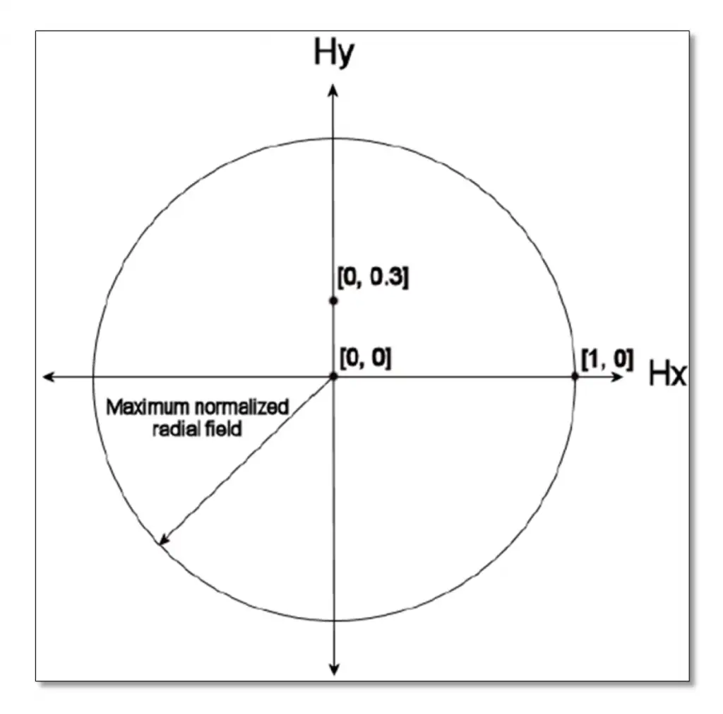
Radial Field Normalization
If the field normalization is radial, then the normalized field coordinates represent points on a unit circle. The radius of this unit circle, called the maximum radial field, is given by the radius of the field point farthest from the origin in field coordinates. The maximum radial field magnitude is then used to scale all fields to normalized field coordinates. Real field coordinates can be determined by multiplying the normalized coordinates, Hx and Hy , by the maximum radial field magnitude:

 and
and 
where Fr is the maximum radial field magnitude and fx and fy are the field coordinates in field units.
For example, suppose 3 field points are defined in the (x, y) directions using object height in lens units at (0.0, 0.0), (10.0, 0.0), and (0.0, 3.0). The field point with the maximum radial coordinate is the second field point, and the maximum radial field is therefore 10.0. The normalized coordinate (Hx = 0, Hy = 1) would refer to the field coordinates (0.0, 10.0). The normalized coordinate (Hx = 1, Hy = 0) would refer to the field coordinates (10.0, 0.0). Note the normalized field coordinates can define field coordinates that do not correspond to any defined field point. The maximum radial field is always a positive value. If a fourth field point at (-10.0, -3.0) were added in the above example, the maximum radial field would become

or approximately 10.44031. Normalized coordinates should always be between -1 and 1, and should also meet the condition:
Otherwise, the field point lies outside of the maximum radial field.
Rectangular Field Normalization
If the field normalization is rectangular, then the normalized field coordinates represent points on a unit rectangle. The x and y direction widths of this unit rectangle, called the maximum x field and maximum y field, are defined by the largest absolute magnitudes of all the x and y field coordinates. The maximum x and y field magnitudes are then used to scale all fields to normalized field coordinates. Real field coordinates can be determined by multiplying the normalized coordinates, Hx and Hy , by the maximum x and y field magnitudes:

where Fx and Fy are the maximum x and y field magnitudes, and fx and fy are the field
coordinates in field units.

For example, suppose 3 field points are defined in the (x, y) directions using object height in lens units at (0.0, 0.0), (10.0, 0.0), and (0.0, 3.0). The field point with the maximum x coordinate is the second field point, and the maximum x field is therefore 10.0. The field point with the maximum y coordinate is the third field point, and the maximum y field is therefore 3.0. The normalized coordinate (Hx = 0, Hy = 1) would refer to the field coordinates (0.0, 3.0). The normalized coordinate (Hx = 1, Hy = 0) would refer to the field point (10.0, 0.0). The normalized coordinate (Hx = 1, Hy = 1) would refer to the field coordinates (10.0, 3.0). Note the normalized field coordinates can define field coordinates that do not correspond to any defined field point. The maximum x and y field are always positive values. If a fourth field point at (-10.0, -3.0) were added in the above example, the maximum x and y field values would not change. Normalized rectangular coordinates should always be between -1 and 1 in the Optical System Conventions and Definitions.
Normalized Pupil Coordinates
Normalized pupil coordinates are often used in both most of the design program and
documentation. There are two normalized pupil coordinates: Px and Py. Normalized pupil
coordinates are convenient because useful pupil locations may be defined in a manner that does not change with the aperture size or position. For example, the normalized pupil coordinate (0.0, 1.0) is always at the top of the pupil, and therefore defines a marginal ray. The normalized pupil coordinate (0.0, 0.0) always goes through the center of the pupil, and therefore defines a chief ray.
The normalized pupil coordinates represent points on a unit circle. The radial size of the pupil is defined by the radius of the paraxial entrance pupil, unless ray aiming is turned on, in which case the radial size of the pupil is given by the radial size of the stop.
For example, if the entrance pupil radius (not diameter) is 8 mm, then (Px = 0.0, Py = 1.0) refers to a ray which is aimed to the top of the entrance pupil. On the entrance pupil surface, the ray will have a coordinate of (x = 0.0 mm, y = 8.0 mm). Note that the normalized pupil coordinates should always be between -1 and 1, and that
A significant advantage of using normalized pupil coordinates is that rays defined in
normalized coordinates remain meaningful as the pupil size and position changes. Suppose prior to optimizing a lens design, a ray set is defined to compute the system merit function. By using normalized coordinates, the same ray set will work unaltered if the entrance pupil size or position or object size or position is changed later, or perhaps even during the optimization procedure.
NSC
Non-sequential Component (NSC) objects are 3D objects used in non-sequential ray tracing.NSC objects can be defined in non-sequential mode and in mixed mode:
NSC objects are defined in non-sequential mode using the Non-sequential Component Editor.
NSC objects are defined in mixed mode using a Non-sequential Component surface in the Lens Data Editor.
Object Space Numerical Aperture
Object space numerical aperture is a measure of the rate of divergence of rays emanating from the object surface. The numerical aperture is defined as the index of refraction times the sine of the paraxial marginal ray angle, measured in object space. The marginal ray defines the boundary of the cone of light diverging from an object point.
Parameter Data
Parameter data values are used to define certain non-standard surface types. For example, parameter data may include aspheric coefficients, grating spacings, or tilt and decenter data.
Paraxial and Parabasal Rays
The term paraxial means “near the axis”. Paraxial optics are optics that are well described by the linear form of Snell’s law. Snell’s law is:

For small angles this becomes
Many definitions in optics are based upon this assumption of linearity. Aberrations are
deviations from this linearity, and so the paraxial properties of optical systems are often
considered the properties the system has in the absence of aberrations. Paraxial rays are traced using formulas which assume the optical surface power is based only upon the vertex radius of curvature, ignoring local linear tilts and higher order curvature of the surface. Paraxial data is computed on a plane tangent to the surface vertex, assuming the vertex radius of curvature is an acceptable approximation to the surface power over the entire aperture of the surface. Certain unusual surface types do not have a paraxial analog, so the real ray tracing calculations are made at these surfaces, even for a paraxial ray in the Optical System Conventions and Definitions.
Many optics design software computes many paraxial entities, such as focal length, F/#, focal position, entrance pupil diameter, and others. These values should be used with caution when the optical system has components which violate the assumption that the vertex curvature is an acceptable approximation to the surface power over the entire aperture of the surface.
For many analysis features, paraxial data is required, typically as a reference against which real rays are measured. To ensure these features work properly, even for optical systems that do not meet the paraxial assumption above, The design software traces “parabasal” rays which are real (real means using Snell’s law explicitly) that make small angles with respect to a reference ray, which is usually an axis or chief ray. The parabasal rays are used to compute the limiting properties of the system as the stop size is decreased, which provides a good estimate of the paraxial properties.
The reason the design software uses parabasal rays rather than paraxial formulas is because many optical systems include non-paraxial components. Non-paraxial means these components are not well described by conventional axial first-order theory. This includes tilted or decentered systems, systems using holograms, diffractive optics, general aspheres, and gradient index lenses.
In summary, paraxial ray data is computed using first order approximations to the surface power for tracing rays, while parabasal rays are real, exact ray traces close to a chief or reference ray. Most paraxial data, such as EFL, F/#, and magnification, use paraxial rays and the data is invalid if the optical system is not well described by the vertex power of every surface.
Most analysis features in the design software use parabasal rays, to allow these features to work with a greater range of optical systems, including those with optical surfaces not well described solely by their vertex surface power.
Paraxial Image Height
The paraxial radial size of the image in lens units of the full field image at the paraxial image surface.
Paraxial Magnification
The radial magnification, being the ratio of paraxial image height to object height. The paraxial magnification is measured at the paraxial image surface. The value is always zero for infinite conjugate systems in most of the Optical System Conventions and Definitions. .
Paraxial Working F/#
The paraxial working F/# is defined as

where θ is the paraxial marginal ray angle in image space and n is the index of refraction of image space. The paraxial marginal ray is traced at the specified conjugates. For non-axial systems, this parameter is referenced to the axis ray and is averaged over the pupil. The paraxial working F/# is the effective F/# ignoring aberrations.
Primary Wavelength
The primary wavelength in micrometers is displayed. This value is used for calculating most other paraxial or system values, such as pupil positions.
Radii
The radius of curvature of each surface is measured in lens units. The convention is that a radius is positive if the center of curvature is to the right (a positive distance along the local z axis) from the surface vertex, and negative if the center of curvature is to the left (a negative distance along the local z axis) from the surface vertex. This is true independent of the number of mirrors in the Optical System Conventions and Definitions.
Real propagation
A real propagation means the rays are propagated in the direction energy would actually flow.
Sagittal and Tangential
The term “tangential” refers to data computed in the tangential plane, which is the plane
defined by a line and one point: the line is the axis of symmetry, and the point is the field point in object space. The sagittal plane is the plane orthogonal to the tangential plane, which also intersects the axis of symmetry at the entrance pupil position.
For typical rotationally symmetric systems with field points lying along the Y axis, the
tangential plane is the YZ plane and the sagittal plane is the plane orthogonal to the YZ plane which intersects the center of the entrance pupil.
The problem with this definition is that it is not readily extended to non-rotationally symmetric systems. For this reason, some design software instead defines the tangential plane to be the YZ plane regardless of where the field point is, and tangential data is always computed along the local y axis in object space. The sagittal plane is the orthogonal to the YZ plane, and intersects the center of the entrance pupil in the usual way, and sagittal data is always computed along the x axis in object space.
The tangential plane and sagittal plane are rotated in pupil coordinates by the Tangential Angle in the Fields section of the System Explorer about the z axis.
The philosophy behind this convention is as follows. If the system is rotationally symmetric, then field points along the Y axis alone define the system imaging properties, and these points should be used. In this case, the two different definitions of the reference planes are redundant and identical. If the system is not rotationally symmetric, then there is no axis of symmetry, and the choice of reference plane is arbitrary.
The size of each surface is described by the semi-diameter setting if it is non-rotationally symmetric and the clear semi-diameter setting if it is rotationally symmetric. The default setting is the radial distance to the aperture required to pass all real rays without clipping any of the rays. Typing a value for the clear semi-diameter or semi-diameter column results in the character “U” being displayed next to the value. The “U” indicates that the clear semi-diameter or semi-diameter is user defined. When a user-defined clear semi-diameter or semi-diameter is placed on a surface with refractive power (which is done by typing in a value in the appropriate column), and no surface aperture has been defined, the design software automatically applies a “floating” aperture to the surface. A floating aperture is a circular aperture whose radial maximum coordinate is always equal to the clear semi-diameter or semi-diameter of the
surface in the Optical System Conventions and Definitions.
Clear semi-diameters on any surface for axial symmetric systems are computed very
accurately, as long as the surface does not lie within the caustic of the ray bundle (note this usually occurs at or near the image surface). The software estimates clear semi-diameters for axial systems by tracing a few marginal pupil rays. For non-axial systems, the software estimates the required clear semi-diameter or semi-diameters using either a fixed number of rays or by an iterative technique, which is slower but more accurate.
It is important to note that the “automatic” clear semi-diameter or semi-diameter
computed by the software is an estimate, although it is generally a very good one.
Some surfaces may become so large in aperture that the surface z coordinate becomes
multiple valued; for example, a very deep ellipse may have more than one z coordinate for the same x and y coordinates on the surface. For the case of spherical surfaces, this condition is called “hyperhemispheric” and the software uses this term even if the surface is not a sphere. Hyperhemispheric surfaces are denoted by an asterisk “*” in the semi-diameter column. The indicated semi-diameter is of the outer edge of the surface, which will have a smaller radial aperture than the maximum radial aperture.
Sequential Ray Tracing
Sequential ray tracing means rays are traced from surface to surface in a predefined sequence. The software numbers surfaces sequentially, starting with zero for the object surface. The first surface after the object surface is 1, then 2, then 3, and so on, until the image surface is reached. Tracing rays sequentially means a ray will start at surface 0, then be traced to surface 1, then to surface 2, etc. No ray will trace from surface 5 to 3; even if the physical locations of these surfaces would make this the correct path.
Special Characters
There are many places in the software where user defined file, material, glass, or other names may be provided. Generally, the software allows any characters to be used in these names, except for a few reserved “special characters” The special characters are space, semi-colon, single quote, and tab.
Strehl Ratio
The Strehl ratio is one commonly used measure of optical image quality for very high quality imaging systems. The Strehl ratio is defined as the peak intensity of the diffraction point spread function (PSF) divided by the peak intensity of the diffraction point spread function (PSF) in the absence of aberrations. The software computes the Strehl ratio by computing the PSF with and without considering aberrations, and taking the ratio of the peak intensity. The Strehl ratio is not useful when the aberrations are large enough to make the peak of the PSF ambiguous, or for Strehl ratios smaller than about 0.1 in the Optical System Conventions and Definitions.
Surface Apertures
Surface apertures include circular, rectangular, elliptical, and spider shaped apertures which can vignette rays. There are also user defined shapes for surface apertures and obscurations; and a “floating” aperture that is based upon the current clear semi-diameter or semi-diameter value. Surface apertures do not affect ray launching or tracing, except for the termination of a ray if it does not pass the surface aperture. Surface apertures have no effect on the system aperture.
System Aperture
The system aperture is the overall system F/#, Entrance Pupil Diameter, Numerical Aperture, or Stop Size. Any of these 4 quantities is sufficient to define the other 3 for a particular optical system. The system aperture is used to define the object space entrance pupil diameter, which in turn is used to launch all rays. The system aperture is always circular. Rays may be vignetted after being launched by various surface apertures. There is only one system aperture, although there may be many surface apertures.
Thicknesses
Thicknesses are the relative distance to the next surface vertex in lens units. Thicknesses are not cumulative, each one is only the offset from the previous vertex along the local z axis. The orientation of the local z axis can change using coordinate breaks or surface tilts and decenters. Thicknesses corresponding to real propagation always change sign after a mirror. After an even number of mirrors (including zero mirrors), thickness are positive for real propagations and negative for virtual propagations. After an odd number of mirrors, thicknesses are negative for real propagations and positive for virtual propagations. This sign convention is independent of the number of mirrors, or the presence of coordinate breaks. This fundamental convention cannot be circumvented through the use of coordinate rotations of 180 degrees.
Total Internal Reflection (TIR)
TIR refers to the condition where a ray makes too large an angle with respect to the normal of a surface to meet the refraction condition as specified by Snell’s Law. This usually occurs when a ray with a large angle of incidence is refracting from a high index media to a lower index media, such as from glass to air. When doing sequential ray tracing, rays which TIR are considered errors, and are terminated. Physically, the ray would reflect rather than refract from the boundary, but the software does not consider this effect when doing sequential ray tracing. For non-sequential ray tracing, rays which TIR are properly reflected.
Total Track
Total track is the length of the optical system as measured by the vertex separations between the “left most” and “right most” surfaces. The computation begins at surface 1. The thickness of each surface between surface 1 and the image surface is considered, ignoring any coordinate rotations. The surface which lies at the greatest z coordinate defines the “right most” surface, while the surface with the minimum z coordinate defines the “left most” surface. Total track has little or no value in non-axial systems.
Vignetting Factors
Vignetting factors are coefficients which describe the apparent entrance pupil size and
location for different field positions. The software uses five vignetting factors: VDX, VDY, VCX, VCY, and TAN. These factors represent decenter x, decenter y, compression x, compression y,and tangential angle, respectively. The default values of all five factors are zero, which indicates no vignetting.
Both the field of view and the entrance pupil of an optical system can be thought of as unit circles. The normalized field and pupil coordinates, defined in “Normalized field coordinates”, are the coordinates on these two unit circles. For example, the pupil coordinates (px = 0, py =1) refer to the ray which is traced from some point in the field to the top of the entrance pupil. If there is no vignetting in the system, The software will trace rays to fill the entire entrance pupil during most computations.
Many optical systems employ deliberate vignetting. This means a portion of the rays are
intentionally “clipped” by apertures other than the stop surface. There are two common reasons for introducing vignetting in an Optical System Conventions and Definitions.
- First, vignetting decreases the size of the lenses, particularly in wide angle lenses.
- Second, vignetting may remove a portion of the beam which would be excessively aberrated.
Vignetting usually increases the F/# as a function field angle (which darkens the image), but the image quality may improve if the most severely aberrated rays are clipped.
Vignetting factors redefine the entrance pupil for a specific field position. The normalized pupil coordinates are modified using two successive transformations. First, the coordinates are scaled and shifted:

The scaled and shifted coordinates are then rotated by the tangential angle, 0:

The VDX term can shift the apparent pupil left and right, while VCX makes the pupil larger or smaller in the x direction. Similar results hold for the VDY and VCY values. Note that if the vignetting factors are all zero, the pupil coordinates are left unmodified. Vignetting factors provide a convenient way of designing optics which employ vignetting. However, there are restrictions to using vignetting factors that must be understood. Some features are capable of tracing rays from arbitrary field positions where no vignetting factors have been assigned. These features may not provide completely accurate results for data computed at field positions other than the defined fields. Some features will remove the vignetting factors for these computations by placing a clear aperture on each surface that vignettes the rays an equivalent amount. Features that automatically remove the vignetting factors are described in the Analysis. Some features do not automatically remove vignetting factors for intermediate field positions, such as ray operands in the merit function (operands like REAX that can launch a single ray, for example) or ZPL macros. If the vignetting factors are not removed, the software will attempt to interpolate the vignetting factors. For rotationally symmetric systems, or systems with field points entirely along the y axis, The software interpolates between adjacent field points to estimate the vignetting factors to use at intermediate field points. For more general optical systems with X field values, the software uses the closest defined field point for determining the vignetting factors for an arbitrary field point in the Optical System Conventions and Definitions.
Once a vignetting factor is defined, it is up to the designer to ensure that rays beyond the apparent pupil are in fact vignetted! If the vignetting factor is used to shrink the size of the lenses, then the lenses should be made no larger than is required to pass the rays which are at the edge of the apparent pupil. If rays from beyond the vignetted aperture are allowed to pass in the real optical system, then the lens performance will not correlate with the computer model. Identical or nearly identical field coordinates may not be defined with different vignetting factors. Field coordinates must be different by roughly 1E-06 times the maximum field coordinate if two neighboring fields use different vignetting factors. This is required because the software must determine vignetting factors for any field coordinates, not just those at defined field positions; and identical field coordinates with different vignetting factors have no physical interpretation. The proper way to set up this sort of system is to use multiple configurations, and change the vignetting factors via the multi-configuration editor.
The vignetting factors work with and without ray aiming turned on. If ray aiming is off, then the paraxial entrance pupil is remapped according to the equations given earlier. If ray aiming is turned on, then the remapping is done at the stop surface.
One possible application of vignetting factors is to account for pupil aberration without using the ray aiming feature. This is an advanced trick which can be used to speed up ray tracing in wide angle systems.
Vignetting factors may be defined on the “Field Data” dialog box.
Vignetting factors may also be zoomable parameters;
Virtual Propagation
A virtual propagation means the rays are propagated in a direction opposite to the direction energy would actually flow. Virtual propagations are often useful for placing virtual sources or pupils.
Wavelength Data
Wavelength data are always measured in micrometers referenced to “air” at the current system temperature and pressure. The default system temperature is 20 degrees Celsius, and the default air pressure is 1.0 atmospheres. If the system temperature and/or pressure is modified, or under the control of multi-configuration operands, care must be taken to adjust the wavelengths to the new air temperature and pressure. Wavelength data are always measured in micrometers referenced to “air” at the system
temperature and pressure.
Working F/#
Working F/# is defined as

where θ is the real marginal ray angle in image space and n is the index of refraction of image space. The marginal ray is traced at the specified conjugates. Working F/# ignores surface apertures but considers vignetting factors.
For off axis field points or non-axial systems, working F/# is determined by the average of the square of the numerical aperture between the axis ray and four marginal rays, at the top, bottom, left, and right side of the vignetted pupil. The average of the square of the numerical aperture of the four rays is converted back to equivalent F/# in the Optical System Conventions and Definitions.
Working F/# is generally much more useful than image space F/# because it is based upon real ray data at the actual conjugates of the lens.
If the marginal rays cannot be traced (due to ray errors) then a smaller pupil is temporarily used to estimate the working F/#. In this case, the software scales the data to estimate the working F/# at the full pupil size, even though rays are not be traceable at the full aperture.
If the marginal rays are nearly parallel to the chief ray, the resulting F/# may become so large as to be inaccurate. The software will automatically “cap” the F/# at 10,000 if the calculated F/# becomes larger than 10,000. This result simply means the F/# cannot be calculated accurately using rays. Such a large F/# means the output beam is nearly collimated, and many assumptions the software makes are not valid in this case. The two solutions are to bring the nearly collimated beam to a focus using a paraxial lens, or to use the exit pupil size and position to estimate the F/#.