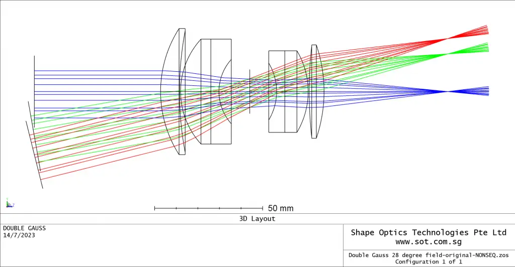
Here, an example, Double Gauss 28 degree field design example will be used to share optical algorithm when Converting sequential surfaces to nonsequential objects
Note: Don’t assume this optical algorithm conversion perfectly converts your sequential surface data; carefully check the non-sequential conversion results before doing any important analysis. you could download the demo example from our server: optical algorithm.

The conversion works by the following algorithm:
1. First a Non-Sequential Component surface and a dummy exit port surface are inserted. The exit port is positioned to coincide with the last surface in the defined range.
2. The range of surfaces is converted into either the corresponding NSC surface objects (for standalone surfaces and mirrors with zero substrate thickness) or NSC objects (for pairs of surfaces with a material between, or mirrors with non-zero substrate thickness).
3. Coordinate breaks are replaced with null objects with equivalent rotations; and subsequent objects will reference the null objects.
4. The original surfaces are then deleted.
5. If the “Convert file to non-sequential mode” box is checked, then the file is placed in non-sequential mode, and any surfaces outside the selected range are deleted.
6. If the “Add Sources & Detectors” box is checked, then each sequential field in the Field Data Editor is converted to a non-sequential Source Ellipse. The parameters of the Source Ellipses are calculated using the sequential field locations and Entrance Pupil Diameter.
7. In addition, the centroid location in this optical algorithm at the IMAGE surface is calculated for each sequential field, using the Spot Diagram analysis. Detector Rectangles are inserted at these centroid locations with comments corresponding to each field number. The Detector Rectangles are the same size as the default display width of the Spot Diagram analysis with “Show Airy Disk” checked-on.
a. For focal systems with a flat image plane, each field point’s Detector Rectangle lies in the same XY plane (assuming the Z axis is the optical axis). For most systems, these Detector Rectangles are small and separated in X & Y so that the
Detector Rectangles do not overlap. If the Detectors do overlap, then the nesting rule will be followed and some detectors may not see all of the rays. In this case, you will need to manually adjust the locations of the detectors, most likely along the optical axis, such that the detectors are separated by more than the “Glue Distance” in the System Explorer.
b. Although curved IMAGE surfaces are not converted into curved detectors, the positions of the Detector Rectangles are calculated using the surface sag and normal angles at the centroid of each field.
c. When “Afocal Image Space” is checked-on in the System Explorer, we assume that the rays are nearly collimated at the IMAGE surface in the Lens Data Editor.
This typically means that the RMS spot size (in um) is large, so the Detector Rectangles for each field point will also be large, and thus are likely to overlap. Therefore, Detector Rectangles for Afocal systems will be offset slightly along the optical axis, by values just larger than the “Glue Distance” in the System Explorer. This offset should not significantly change the results if the rays are nearly collimated.


A Detector Color is also added, and is located slightly after the Detector Rectangle(s). It is offset by a distance just larger than the “Glue Distance” in the System Explorer. The size of the Detector Color is determined by the default display width of the sequential Full Field Spot Diagram analysis.
9. For focal systems at finite conjugates (where the OBJECT is not at infinity), an inactive Source DLL “Lambertian Overfill” and a Slide object are also inserted just before the field point Source Ellipses. The Source DLL and Slide object can be used to test the imaging quality of the system:
a. The sizes of the Source DLL and Slide object are determined by the Clear Semi- Diameter of the OBJECT surface in the Lens Data Editor.
b. The Source DLL “Lambertian Overfill” will overfill the first aperture of the sequential system with a Lambertian distribution. The distance from the Source DLL to the first aperture is defined by the “Target Distance” parameter. The diameter of the first aperture is given by the “Target Diameter” parameter, and note that this target aperture must be circular. The size of the Source DLL is given by the “Source Width” and “Source Height” parameters, but unlike the target aperture, the source area may be elliptical or rectangular. For the non-sequential conversion, the Source DLL is square so that it matches the dimensions of the Slide Object.
c. The Source DLL rays originate from a uniform spatial distribution within the square source area. A circular right cone is fit around the virtual target aperture, and the ray direction is then randomly chosen from a uniform angular distribution within this cone. Because the circular cone is slightly larger than the elliptical cross-section of the target aperture, the ray may end up slightly outside the circular target aperture. Therefore, the target aperture will end up being overfilled, generally by a modest amount. See “Source DLL” for more information about the Lambertian Overfill source DLL.
10 If the IMAGE surface in the Lens Data Editor has a Material defined, then an additional object is added to the non-sequential file, which starts at the location of the sequential IMAGE surface. The back face of this object is not defined (because the IMAGE surface is always the last surface in the LDE), so the radius and clear aperture of the back face are picked up from the front face, and the thickness is 1 lens unit.
a. With this additional object representing the material after the IMAGE surface, placement of the Detector Color becomes ambiguous. Therefore, if the IMAGE surface has a Material defined, then the sequential file will be converted to nonsequential mode without the Source DLL, Slide Object, and Color Detector.
11. Note that unless the “Save New System As…” box is checked on; the converted nonsequential file will overwrite the current sequential file. This action cannot be undone in this optical algorithm.
The feature of this optical algorithm may not work correctly in all cases. Some additional dummy surfaces with small spacings may need to be inserted prior to and after the range of lens surfaces to be converted.