How to simulate laser – fibre coupling, how to setup and simulate the fiber optics propagation? This article demonstrates how to set up a laser fiber coupling system using Physical Optics Propagation.
In this sharing section, we describe a commercial fiber coupler, which couples Corning HI 1060 Fiber using an commercial end cap, and then an collimating lens collimate the fiber beam.

The manufacturers’ data is as follows.
|
Single Mode Fiber, Corning RCHi 1060 |
|
|
Numerical Aperture |
0.14 |
|
Core Diameter |
5.3 µm |
|
Mode Field Diameter @ 1.06 µ |
6.2± 0.3 µm |
|
End Cap Specs: |
|
|
Substrate material |
Fused Silica |
|
Substrate Size |
1.6mm x 8mm |
|
Internal Transmission |
>0.99 |
First, let’s see and study the fundamentals fiber optics, the Single-Mode Fiber Coupling calculation
The Single-Mode Fiber Coupling calculation provides a more powerful capability for fiber optics with Gaussian-shaped modes. It performs two calculations: an energy-transport calculation and a mode-matching calculation. The system efficiency, S, is the sum of the energy collected by the entrance pupil which passes through the optical system, accounting for both the vignetting and transmission of the optics (if polarization is used), divided by the sum of all the energy which radiates from the source fiber:

where Fs(x,y) is the source fiber amplitude function and the integral in the numerator is only done over the entrance pupil of the optical system, and t(x,y) is the amplitude transmission function of the optics.
Aberrations in the fiber optics system introduce phase errors which will affect the coupling into the fiber. Maximum coupling efficiency is achieved when the mode of the wavefront converging towards the receiving fiber perfectly matches the mode of the fiber in both amplitude and phase at all points in the wavefront. This is defined mathematically as a normalized overlap integral between the fiber and wavefront amplitude, T:

where Fr(x,y) is the function describing the receiving fiber complex amplitude, W(x,y) is the function describing the complex amplitude of the wavefront from the exit pupil of the optical system, and the ‘ symbol represents complex conjugate. Note that these functions are complex valued, so this is a coherent overlap integral. T has a maximum possible value of 1.0, and will decrease if there is any mismatch between the fiber amplitude and phase and the wavefront amplitude and phase.
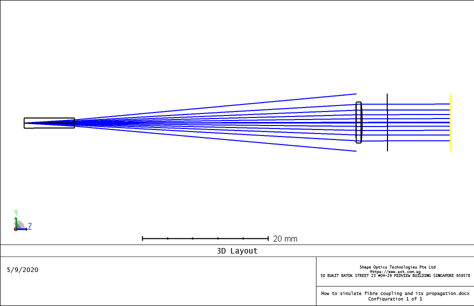
Go back our sharing example, the setup and layout of the example are as below, and you could download the design file at the end of this article.

Please be noted:
- Be wary of the multiple definitions of the term “numerical aperture” in the fiber optics. It may use the sine of the marginal ray angle, the sine of the angle at which the intensity has fallen to 1/e2 (both definitions are used in different calculations, as we shall see) or the sine of the angle at which the intensity has fallen to 1% of peak, as used by Corning. Definitions matter!
- A Gaussian apodization has been applied to the aperture definition to highlight the Gaussian distribution of light. This is currently only approximate. The calculations we shall use later will be precise
In this calculation, the source modes are defined by their fibre optics NA, which is defined as the refractive index n of the object or image space surfaces times the sine of the half-angle to the 1/e2 power point. This angle can be computed in one of two ways:
- From the divergence angle of the Gaussian beam calculation, using the mode field diameter to define the beam waist (as in the previous example).
- From the 1% power NA given in the Corning datasheet, and computing the 1/e2 power point from that.
The mode field diameter of the fiber optics at wavelength 1.06 µm is 6.2 ± 0.3 µm according to the Corning datasheet. Let’s check the Paraxial Gaussian Beam and set up the analysis as follows.

The beam waist is always positioned relative to Surface 1, which in this case is positioned at the same place as the object surface. Therefore, a Gaussian waist radius of 3.1 µm is positioned at the source fiber location. It then propagates through the optical system.
The single mode fibre optics coupling and propagation calculation can be significantly expanded by using Physical fiber Optics Propagation (POP). The coupling is still computed by an overlap integral, but the use of Physical Optics gives major benefits:
- Any complex mode can be defined; the calculation is not restricted to Gaussian modes.
- Diffraction effects due to the beam being truncated on apertures, or due to propagation over long distances, can be accurately modelled.
The beam width at surface 7, or image surface as below:
We could see and compare fiber optics propagation intensity, beam size, M2 etc by POPD operant:
Beam width simulated by paraxial Gaussian beam analysis is: 5.56mm, while beam width simulated by POP is 3.04mm, which is more accurate.
Let’s check the phase @ the image surface, Note the shape of the phase profile, which shows parabolic and quartic terms: equivalent to focus and spherical aberration. Note also the truncation of the phase profile at the edge of the lens.
The POPD reports all the Physical fibre Optics data via the Merit Function Editor, and is often a more useful reference.

The design file used in this particle is attached, please download it here.How to simulate fibre coupling and its propagation
Reference Source:
- https://www.zemax.com/
- Zemax Optical Design Program User’s Guide, Zemax Development Corporation
- https://en.wikipedia.org/wiki/Main_Page
- https://www.corning.com/media/worldwide/csm/documents/HI%201060%20Specialty%20Fiber%20PDF.pdf
- https://www.machinemfg.com/fiber-laser-cutting/