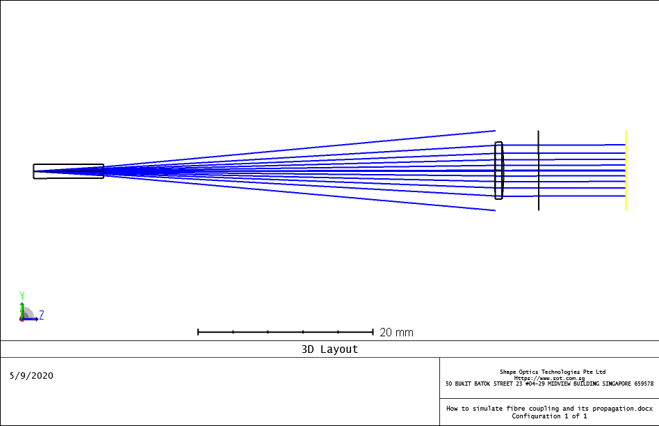
Accurate simulation of laser–fiber coupling and fiber propagation is critical for high-performance photonic systems. This article demonstrates how to set up a laser–fiber coupling model using Physical Optics Propagation (POP), which captures diffraction, truncation, and phase effects that are missed by simple paraxial methods.
We use a commercial fiber coupler that launches light into a single-mode fiber via a commercial end cap, followed by a collimating lens that collimates the output beam.

Fiber and End-Cap Specifications
Single-Mode Fiber: Corning RCHi 1060
- Numerical Aperture (NA): 0.14
- Core Diameter: 5.3 µm
- Mode Field Diameter @ 1.06 µm: 6.2 ± 0.3 µm
End Cap:
- Material: Fused silica
- Size: 1.6 mm × 8 mm
- Internal Transmission: > 0.99
Fundamentals: Single-Mode Fiber Coupling
Single-mode fiber coupling for Gaussian-like modes involves two complementary calculations:
1) Energy Transport (Throughput)
The system efficiency SS is the fraction of source energy that passes through the entrance pupil and optical train (including vignetting and transmission):

where Fs(x,y) is the source fiber amplitude and t(x,y) is the optics’ amplitude transmission.
2) Mode Matching (Overlap Integral)
Maximum coupling occurs when the amplitude and phase of the incident wavefront match the fiber mode. The normalized coherent overlap is:

where Fr(x,y) is the function describing the receiving fiber complex amplitude, W(x,y) is the function describing the complex amplitude of the wavefront from the exit pupil of the optical system, and the ‘ symbol represents complex conjugate.
Note that these functions are complex valued, so this is a coherent overlap integral. T has a maximum possible value of 1.0, and will decrease if there is any mismatch between the fiber amplitude and phase and the wavefront amplitude and phase.

Practical Notes on Numerical Aperture (NA)
Be careful: “NA” has multiple definitions in fiber optics.
- nsinθ at the 1/e² intensity point (common in Gaussian optics)
- nsinθ at 1% intensity (used by some manufacturers, including Corning)
Definitions matter. Conversions between 1% and 1/e² must be done consistently.
A Gaussian apodization may be applied to visualize the mode, but the POP calculations below are exact, not approximate.
Defining the Source Mode
The source mode can be defined in two consistent ways:
- From Gaussian beam divergence, using the mode field diameter (MFD) to set the waist.
- From the 1% NA in the datasheet, converted to the 1/e² point.
For RCHi 1060 at 1.06 µm, MFD = 6.2 µm, so the waist radius is 3.1 µm.
Place the Gaussian waist at the source fiber plane (Surface 1), then propagate through the system.

The beam waist is always positioned relative to Surface 1, which in this case is positioned at the same place as the object surface. Therefore, a Gaussian waist radius of 3.1 µm is positioned at the source fiber location. It then propagates through the optical system.
Why Physical Optics Propagation (POP)?
While Gaussian/paraxial methods are fast, POP provides decisive advantages:
- Supports arbitrary complex modes (not limited to Gaussian)
- Accurately models diffraction from apertures and long propagation distances
- Captures phase (focus, spherical aberration) and truncation effects
- Computes coupling via coherent overlap with the fiber mode
Results: POP vs Paraxial Gaussian
At the image surface (Surface 7):
- Paraxial Gaussian beam width: 5.56 mm
- POP beam width: 3.04 mm (more accurate)
Phase analysis reveals parabolic (focus) and quartic (spherical aberration) terms, plus clear edge truncation at the lens—effects that directly reduce coupling if uncorrected.
The POPD operand reports beam width, intensity, phase, and M^2 via the Merit Function Editor, making it an excellent reference for optimization.

Takeaways and Best Practices
- Use Gaussian/paraxial methods for quick feasibility checks.
- Use POP for final design, tolerance studies, and when apertures/aberrations matter.
- Always confirm NA definitions and spectral wavelength.
- Optimize phase as well as amplitude at the receiving fiber for maximum coupling.
Reference Source
- https://www.zemax.com/
- https://www.corning.com/media/worldwide/csm/documents/HI%201060%20Specialty%20Fiber%20PDF.pdf
- https://www.machinemfg.com/fiber-laser-cutting/
- The design file used in this article is attached as shown. How to simulate fibre coupling and its propagation