This article describes the use of Gaussian Quadrature sampling for determining the optimal set of wavelength spectrum to use in optimizing an optical system for performance over a broad input spectrum.
Introduction
OpticStudio has used GQ sampling of the pupil for optimization of systems since its initial development. In this article, we will show how it is used to accurately model broad wavelength spectrums.
Using GQ wavelength spectrum sampling in OpticStudio
The GQ algorithm developed by Drs. Bauman and Xiao has since been incorporated directly into OpticStudio.
To choose wavelengths spectrum using GQ sampling, the user needs to specify the wavelength range of interest and the number of wavelengths desired:

As always, wavelength spectrum values are in microns. The number of wavelengths – or Steps – that can be chosen can be any even number from 2 to 12. Once the “Gaussian Quadrature” button is selected, OpticStudio will calculate the appropriate wavelengths and weights to characterize the source over the input wavelength range. For example, using four wavelengths to characterize a source over the range of 0.4 to 0.7 microns results in:

The input values for the minimum and maximum wavelength are identical to those provided by the user, within round-off error. Note that OpticStudio will always reset the wavelength range in the GQ dialog box based on minimum and maximum wavelengths defined in the system (this is true regardless of how those wavelengths were defined). Also note that OpticStudio uses a suitable “middle” wavelength as the Primary wavelength, but this can be changed by the user at any time.
Evaluating the RMS spot size of an apochromat
In this section an example (Apochromat3.zmx) is provided to illustrate the benefit of GQ sampling for wavelengths.
To start, open the sample file “Apochromat3.zmx” provided in the server attached. Then add a small off-axis field point to the system:

The performance of this system will be evaluated over the wavelength spectrum range of 0.4-0.7 microns. We’ll start by using four wavelengths uniformly spaced and weighted to define this range. Open the Wavelength Data dialog box and enter:

A plot of the RMS spot size vs. field can be generated under Analyze…RMS…RMS vs. Field.
For the settings shown below, hit the “Save” button (for later use). The results show:

How sensitive are these results to our wavelength spectrum sampling? We can increase the number of wavelengths systematically and then re-evaluate the system to find out. This process has been automated using a ZPL macro. The macro is provided as an attachment.
The basic structure of the macro is as follows:
- Load the lens file
- Change the number of wavelengths and the wavelength values (weights always = 1)
- Retrieve values for the RMS spot size vs. field using the GETTEXTFILE keyword
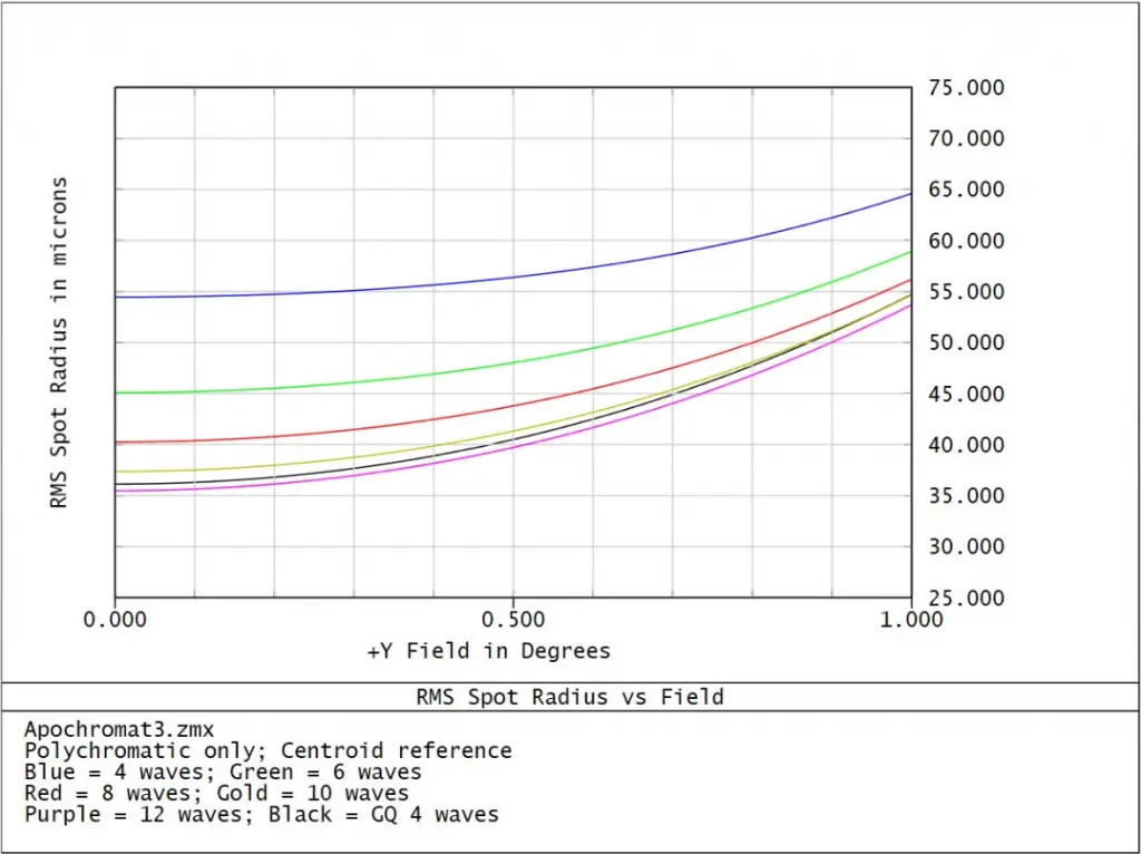
The macro is used to investigate the results for RMS spot size vs. field for 4, 6, 8, 10, and 12 wavelengths. In all cases, the spacing between wavelengths spectrum is constant making the sampling uniform. The macro is then used to compare the results to those generated using four wavelengths (and weights) given by GQ sampling. The results are then plotted using the PLOT keyword:

The data shown above represent the polychromatic results for the 6 cases considered (blue curve = 4 wavelengths; green = 6 wavelengths; red = 8 wavelengths; gold = 10 wavelengths; purple = 12 wavelength; black = GQ with 4 wavelengths). Note how the results generated by uniform wavelength sampling converge towards those generated by GQ sampling. For this system, the results indicate that we would need three times as many uniform wavelengths spectrum to achieve the same level of accuracy as provided by GQ sampling.
Points to consider
As indicated here for wavelength sampling works well for glasses whose dispersion is given by the Sellmeier formula (e.g. glasses from the Schott and Ohara catalogs) and for glasses whose principle absorption occurs near 0.1 microns (the algorithm uses this absorption peak as a reference). Thus, this algorithm may not be appropriate for systems containing dissimilar materials with varying dispersion characteristics or for systems containing materials with significant absorption at longer wavelengths. In addition, this algorithm may be less effective for systems operated at wavelengths longer than about 1.5 microns, since the effect of the IR absorption line will become significant under such conditions.
The effects of wavelength spectrum sampling will generally be significant in systems dominated by chromatic effects. One way to characterize this is to look at Analyze…Aberrations…Chromatic Focal Shift.
Re-open “Apochromat3.zmx” and change the minimum and maximum wavelength to 0.4 and 0.7 microns, respectively. The Chromatic Focal Shift in this system is given by:
When the variation in back focal length with wavelength has a complex structure, as shown above, it will be difficult to characterize such structure with a few uniformly-sampled wavelengths. Under such conditions, GQ sampling will be a much more efficient method of characterizing the wavelength dependence of the system.