This article explains how to tolerance surface irregularities on aspherical components, and how both the spatial frequency of the surface error and its RMS amplitude affect the transmitted wavefront.
Challenges in Tolerancing Aspheric Surface Irregularity
Tolerancing surface irregularity on aspherical components is inherently challenging because surface errors are not deterministic. In practice, the RMS surface error introduced during manufacturing is often specified by the lens supplier as either:
- The measured RMS value from a single representative sample, or
- A statistical average taken from a batch of components.
It is common to hear statements such as a surface being “flat to λ/10” or “λ/20.” However, as will be shown, RMS error alone is insufficient to fully describe optical performance. The spatial frequency of the surface irregularity plays a critical role.
RMS Surface Error Tolerancing Using TEZI
Tolerancing RMS surface error can be performed straightforwardly using the TEZI tolerance operand, provided the following assumptions are valid:
- The nominal surface type is Standard, Even Asphere, or Toroidal.
- The surface error can be reasonably represented using Zernike polynomials.
This assumption is generally valid when surface measurements are obtained via interferometry, since interferometer software typically reports the deviation between the measured surface sag and the nominal surface using a finite set of Zernike terms.
When Standard or Even Asphere surfaces are used in the nominal optical model, the software replaces them with Zernike Standard Sag surfaces during tolerancing. These surfaces retain the same nominal base shape, while the Zernike coefficients describe deviations from that ideal surface.
RMS Amplitude vs. Surface Shape
It is important to note that the RMS amplitude of surface irregularity does not uniquely define the surface shape. Many different surface profiles can share the same RMS value but differ significantly in spatial frequency content.
Example: TEZI Tolerancing Workflow
To illustrate the use of the TEZI operand, consider a simple example. Open the included lens file tolerance_asphere.ZMX, which operates in afocal image space mode and represents a flat optical window. A flat surface is chosen for simplicity, though the same approach applies to any supported aspheric surface.


In the Tolerance Data Editor:
- A tolerance of 1 μm RMS surface error is applied to surface 2.
- The minimum tolerance value is automatically set to the negative of the maximum value to allow both positive and negative Zernike coefficients.
- The resulting RMS surface error is always a positive quantity equal to the specified tolerance magnitude.

Controlling Spatial Frequency with Zernike Terms
The MIN# and MAX# parameters define the range of Zernike terms used:
- Lower-order terms produce low-spatial-frequency errors with broad, smooth surface variations.
- Higher-order terms introduce high-spatial-frequency errors with many localized peaks and valleys (“bumps”).
These limits should be chosen based on interferometric measurements of actual manufactured surfaces, selecting the Zernike order range that best represents the manufacturing process.
The first Zernike term corresponds to piston, which is ignored by optical software; therefore, the minimum allowable value for MIN# is 2. While the maximum possible Zernike term index is 231, practical applications rarely require more than ~28 terms.


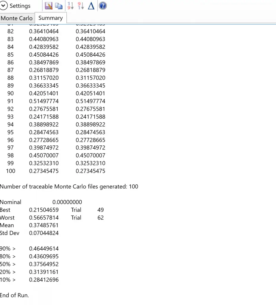
Monte Carlo Tolerancing Results
After running the Monte Carlo tolerancing analysis, the tolerance report provides statistical results for the selected performance metric, such as RMS wavefront error.
Opening a saved Monte Carlo file (e.g., MC_T0001.ZMX) reveals that surface #2 has been converted to a Zernike Standard Sag surface in the Lens Data Editor. Viewing the Surface Sag analysis clearly shows the introduced surface irregularity.
Repeating the tolerance analysis with a higher MAX# value (e.g., 27) results in a surface with significantly more high-frequency features. This demonstrates how the number of Zernike terms directly controls the spatial frequency of the aspheric surface error.
Key Insight: RMS Alone Is Not Enough
This leads to an important conclusion:
As a surface is polished from λ/5 to λ/10, λ/20, or even λ/50, the RMS surface deviation decreases, but the spatial frequency of the remaining irregularity often increases.
Lower-quality surfaces tend to exhibit slow, low-frequency figure errors, while super-polished surfaces often contain high-spatial-frequency micro-structure. Optical performance depends not only on the RMS amplitude of the error but also on the local surface slope, since it is the slope of the surface that ultimately deflects rays and degrades wavefront quality.